ThoughtSpot Tutorials for Snowflake Partner Connect
Explore these tutorials to learn how to model your data after connecting to your Snowflake database.
When you create a connection to Snowflake in ThoughtSpot, any data modeling or table joins are inherited automatically.
If there are no table joins in your Snowflake connection, you can easily create them in ThoughtSpot.
The following example shows how the table joins were created in the Sales table of the Retail Sales worksheet, available in your try.thoughtspot.com account created through Snowflake Partner Connect.
Creating table joins
The joins in the Sales table were created by doing the following:
-
Select Data in the top navigation bar.
-
Select the Tables tab at the top of the page.
-
Select the Sales table.
The Columns view of the Sales table appears.
-
Select the Joins tab.
-
Select +Add join.
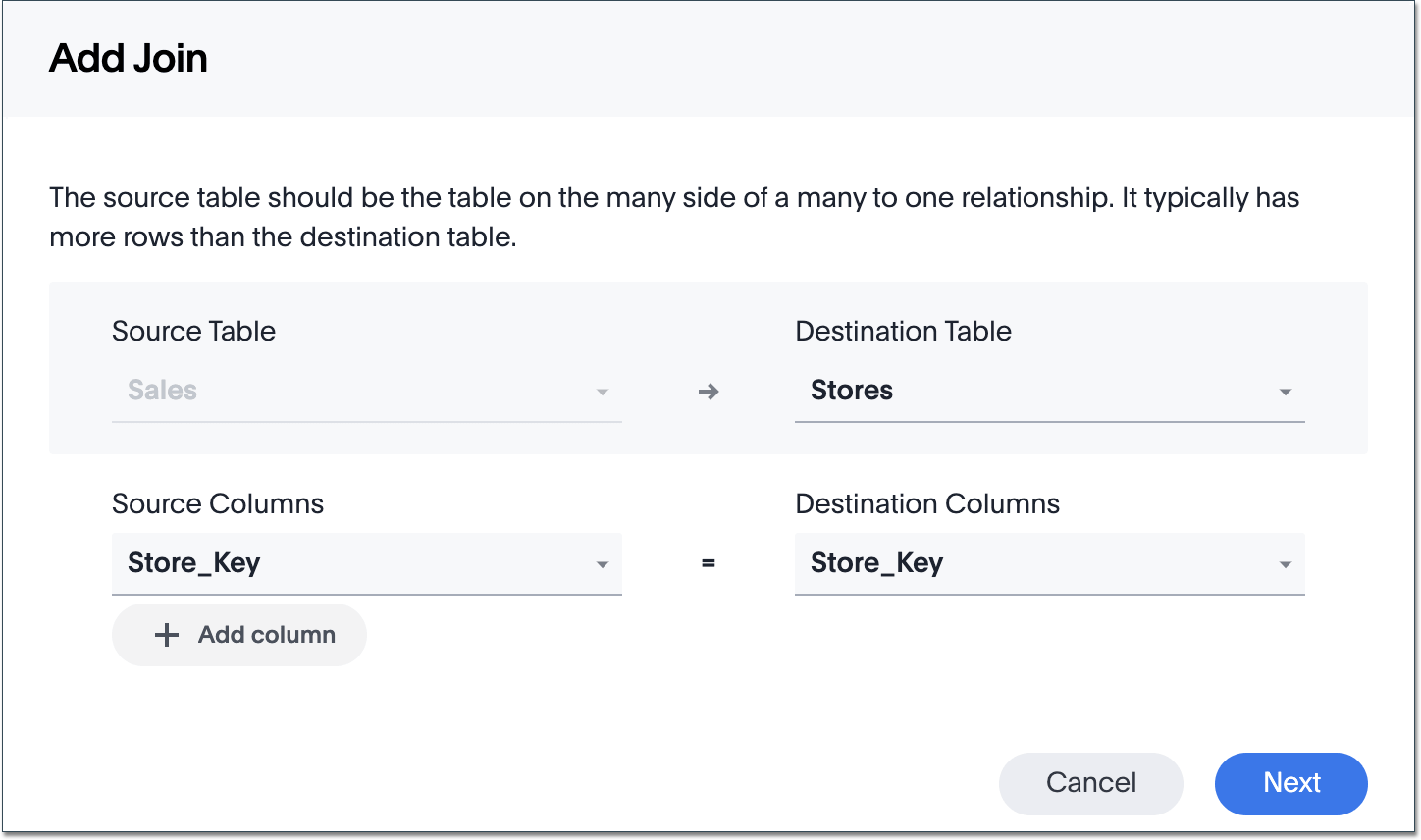
The Add Join window appears.
-
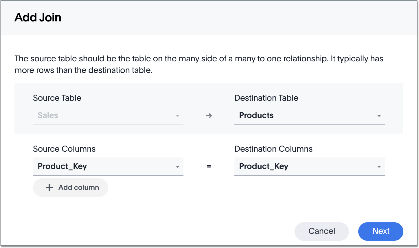
In the Add Join window, use the dropdown menus to make the following selections:
-
For Destination Table, select Products.
-
For Source Columns, select Product_Key.
-
For Destination Columns, select Product_Key.
-
-
Select Next.
-
Enter the name Product_Key - Product_Key, a description for your join (optional), and select Next.
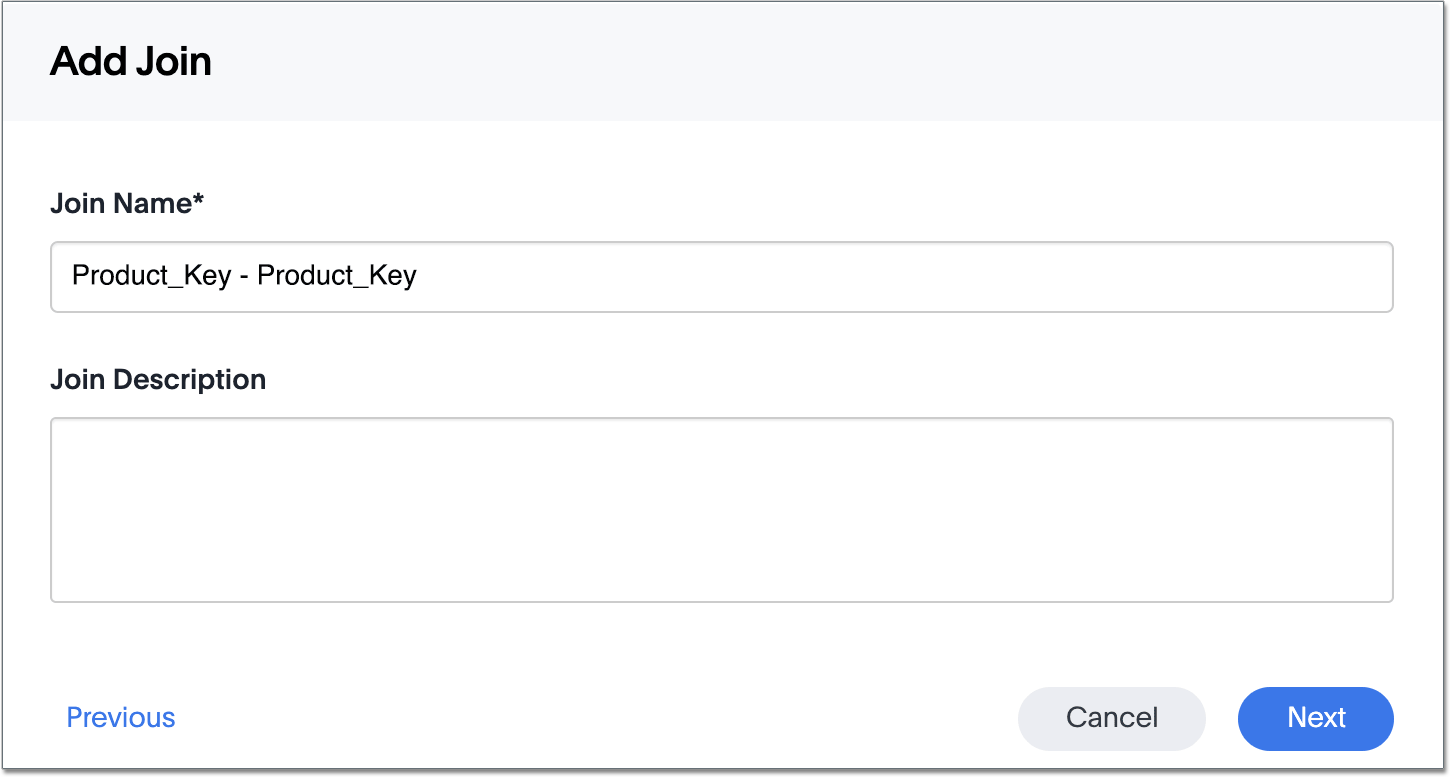
You can use any name you want. The names we’ve chosen for this tutorial match those in the actual schema for this dataset on try.thoughtspot.com. The first join is created. Now you will add the other joins.
-
Select +Add join.
-
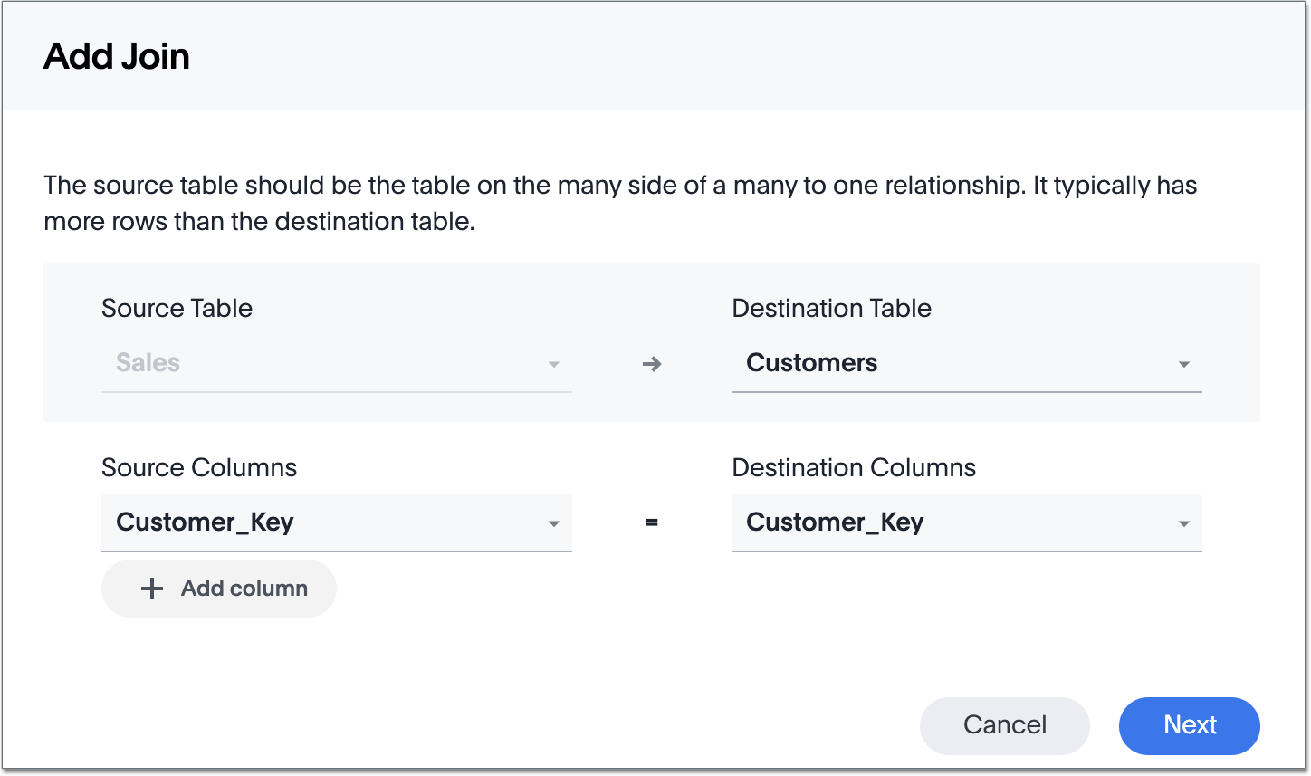
In the Add Join window, use the dropdown menus to make the following selections:
-
For Destination Table, select Customers.
-
For Source Columns, select Customer_Key.
-
For Destination Columns, select Customer_Key.
-
-
Select Next.
-
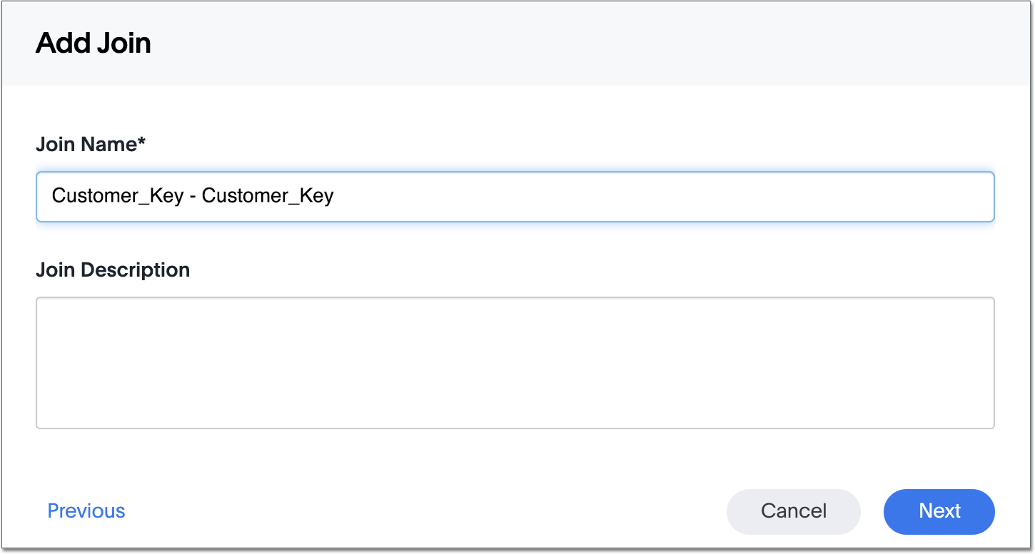
Enter the name Customer_Key - Customer_Key, a description for your join (optional), and select Next.
-
Select +Add join.
-
In the Add Join window, use the dropdown menus to make the following selections:
-
For Destination Table, select Stores.
-
For Source Columns, select Store_Key.
-
For Destination Columns, select Store_Key.
-
-
Select Next.
-
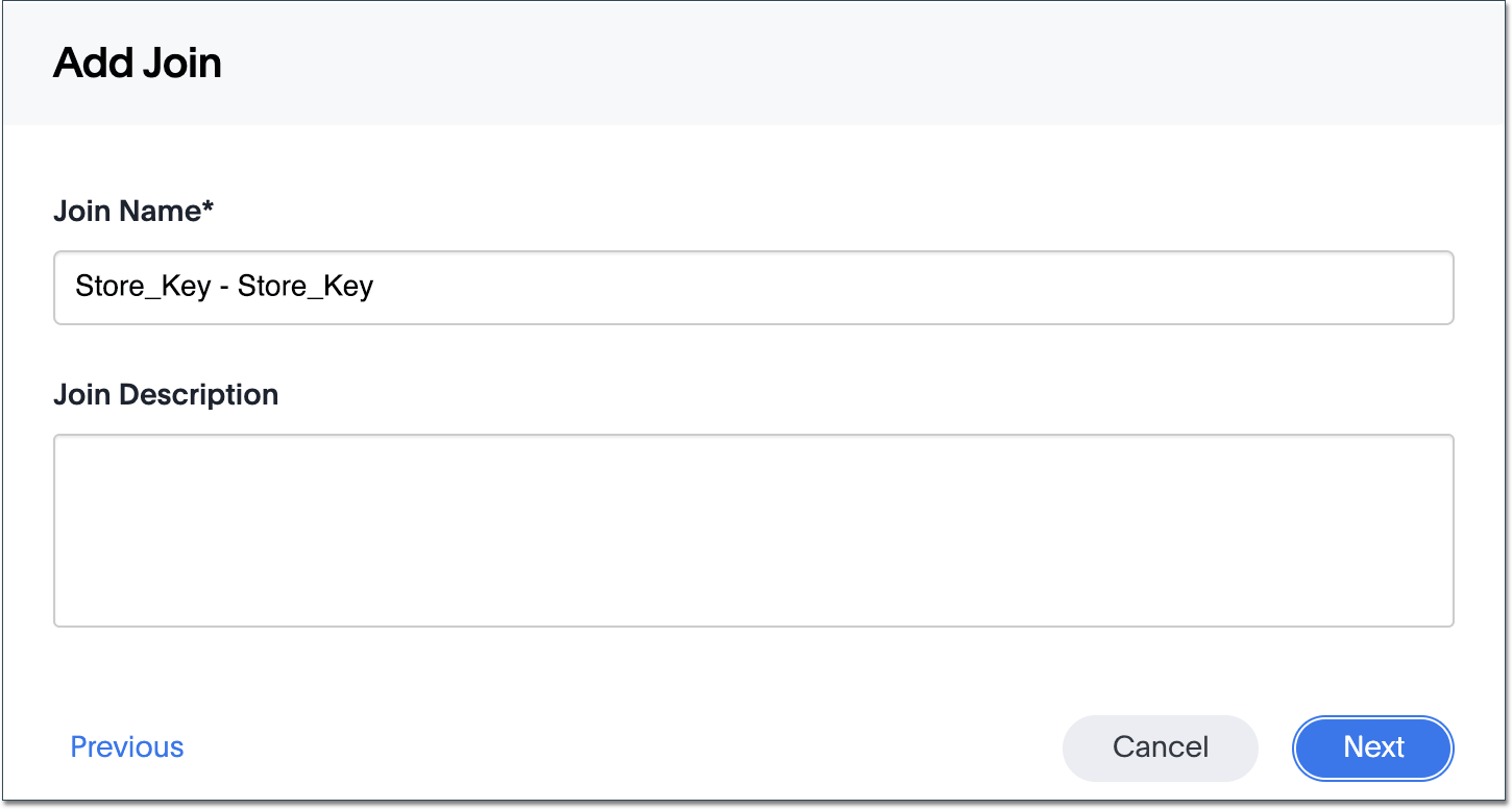
Enter the name Store_Key-Store_Key, a description for your join (optional), and select Next.
-
Select +Add join.
-
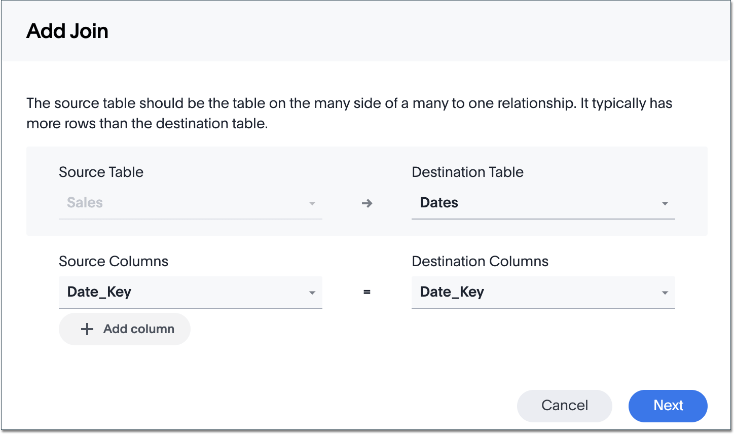
In the Add Join window, use the dropdown menus to make the following selections:
-
For Destination Table, select Dates.
-
For Source Columns, select Date_Key.
-
For Destination Columns, select Date_Key.
-
-
Select Next.
-
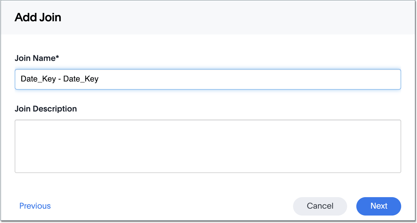
Enter the name Date_Key - Date_Key, a description for your join (optional), and select Next.
Now that all four table joins are created, the schema looks like this:
image::snow-schema.png[A star schema, with the Sales table in the middle. It has arrows pointing out to the Dates, Products, Stores, and Customers tables.]
Searching joined tables
You can easily search the joined tables, without having to create a worksheet.
To search the joined tables, do the following:
-
Select Search.
-
Select the Retail Sales data source, and select Choose sources.
-
Select all the tables you just joined (Customers, Dates, Products, Sales, and Stores) and click Close.
-
In the search bar, enter sales_dollar_amount, store_region, and monthly Date in Dates.
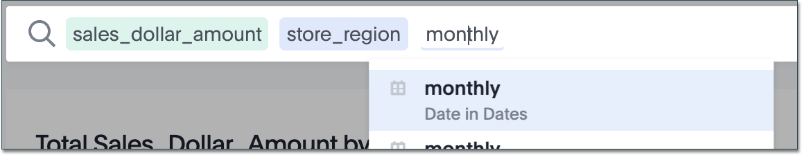
The search results look like this:
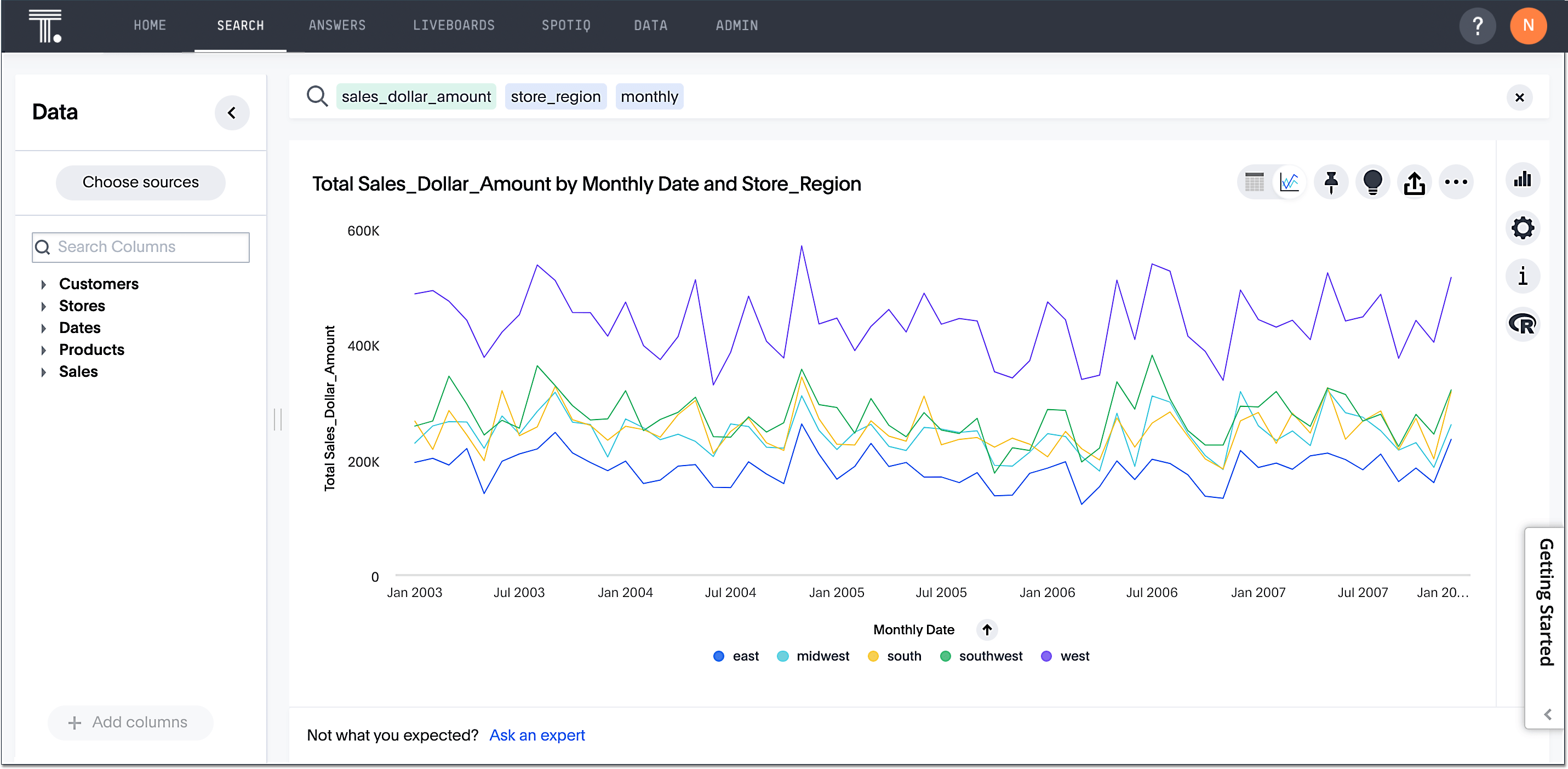
When Monthly is a native keyword, it will work on any timestamp. For the purposes of this example, we’re using monthly as the date, from the Dates table. -
To confirm that the search is honoring the table joins, select the Query details icon
 , to the right of the chart.
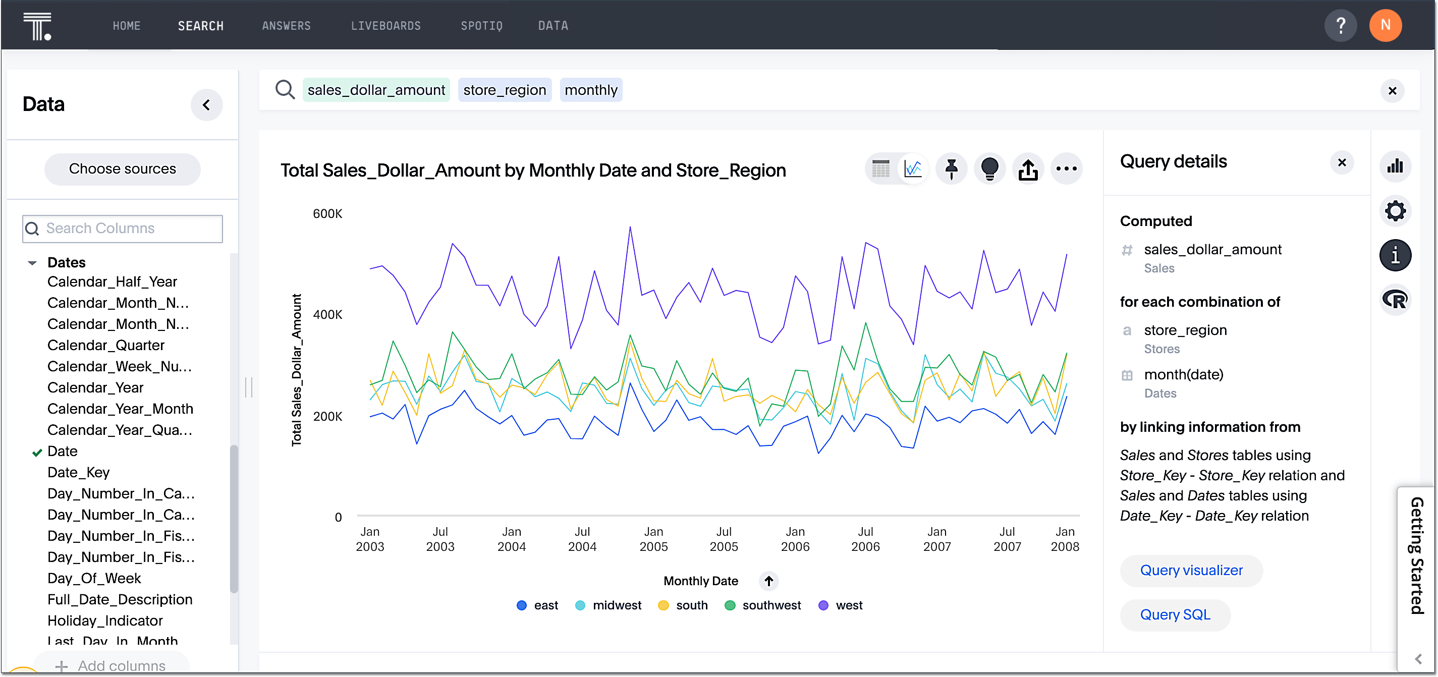
-
To confirm the search is bridging three different tables to create a result, select Query visualizer.
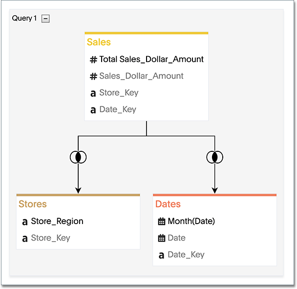
Best practices for data modeling
Here are some examples of how you can model your data to enhance searchability:
-
Change column names
-
Add synonyms for columns
In the following example, the Sales_Dollar_Amount column was renamed to Sales and the synonyms of Revenue and Dollars were added.
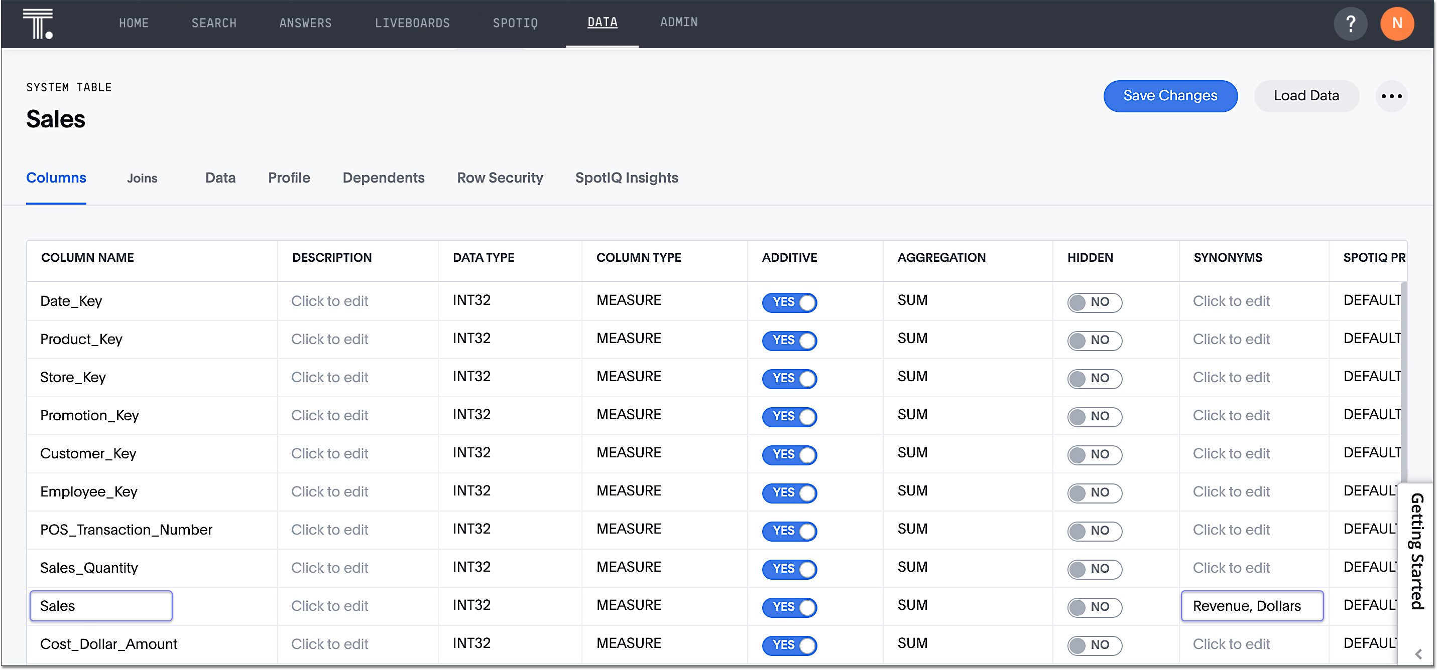
These are just a couple of examples of things you can do.
For more information about data modeling, see: Overview of data modeling settings.
Creating a worksheet
A worksheet is a curated dataset built for ad hoc analysis, that allows you to translate data from a database into the language of your business users.
Examples of things you can do in a worksheet include:
-
Removing columns that aren’t needed
-
Adding data labels and synonyms
-
Adding calculations, such as margin
The worksheet based on the Sales table on try.thoughtspot.com was created by doing the following:
-
Select Data.
-
Select the + Create new button, and select Worksheet.
-
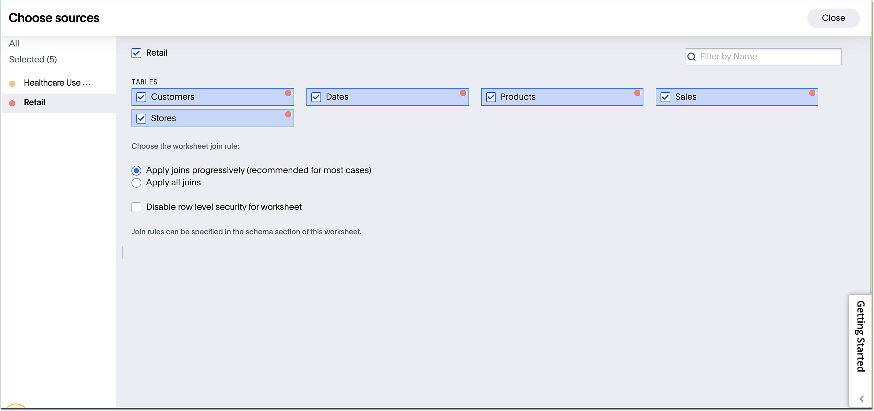
Select the + icon, next to Sources.
-
Check the box next to all five of the tables from the Retail dataset in your schema.
-
Make sure the default setting of Apply joins progressively is selected. This ensures that the search uses only the tables that are required.
-
Select Close.
-
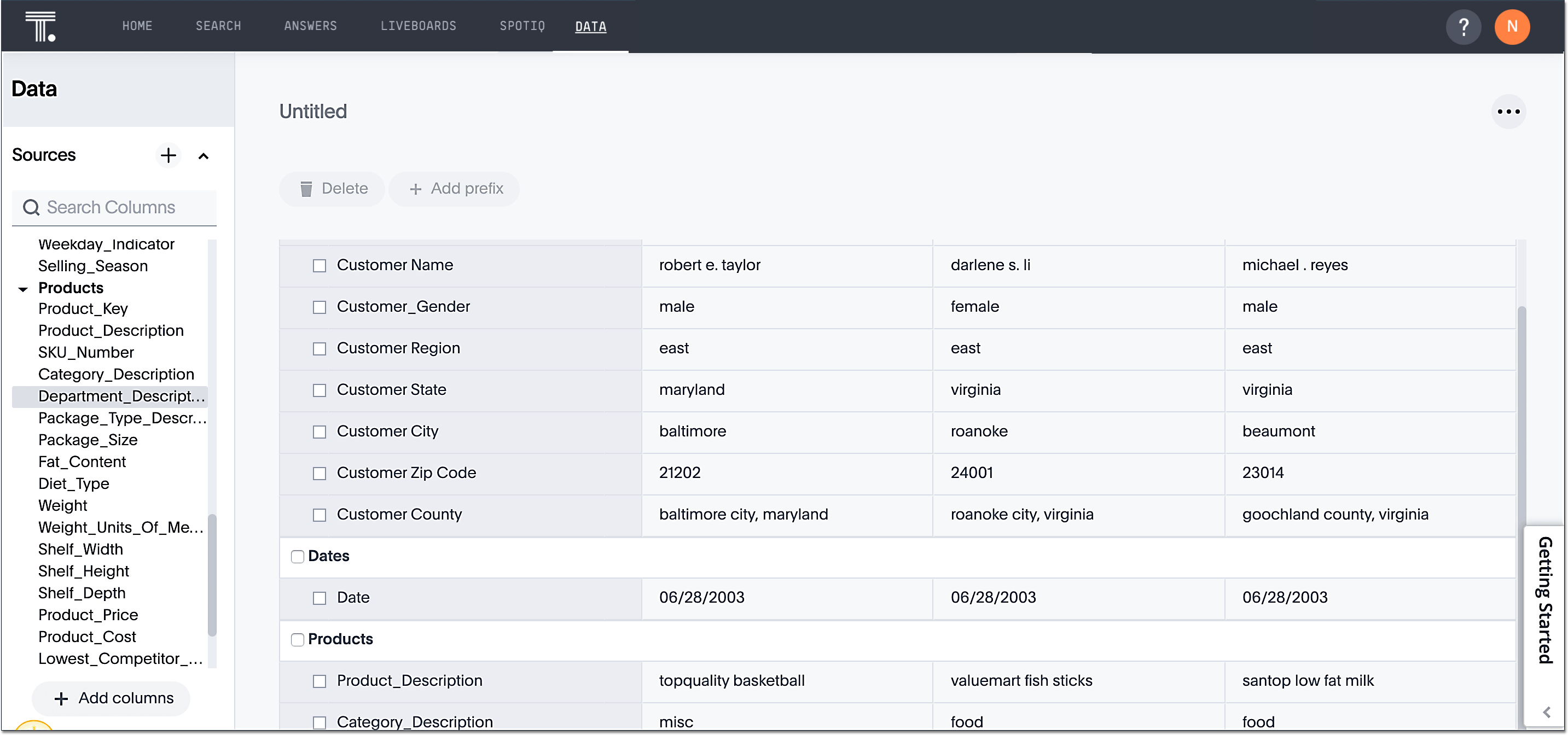
In the Data view, select the name of the Customers table to reveal all of the columns in that table.
-
Double-click each column from the Customers table that you want to include in the worksheet.
Include these columns:
-
Customer_Type
-
Customer Name
-
Customer_Gender
-
Customer Region
-
Customer State
-
Customer City
-
Customer Zip Code
-
Customer County
-
-
Use the same process to select columns from the other tables to include in the worksheet.
From the Dates table, include this column:
-
Date
From the Products table, include these columns:
-
Product_Description
-
Category_Description
-
Department_Description
From the Sales table, include these columns:
-
Sales_Dollar_Amount
-
Cost_Dollar_Amount
-
Gross_Profit_Dollar_Amount
From the Stores table, include these columns:
-
Store_Name
-
Store_Region
-
Store_State
-
Store_City
-
Store_Zip_Code
-
Store_County
As a best practice, you wouldn’t select a key from a table when creating a worksheet, because you wouldn’t want to search for the key. -
-
Select the pencil icon
 next to the current name of your worksheet, enter the name Retail Sales, and click Done.
 -
Select the more options icon
 , and select Save.
Now, let’s add a percent gross margin formula to the worksheet.
-
Select Edit Worksheet.
-
Next to Formulas, select the plus icon
 .
. -
In the formula window, do the following:
-
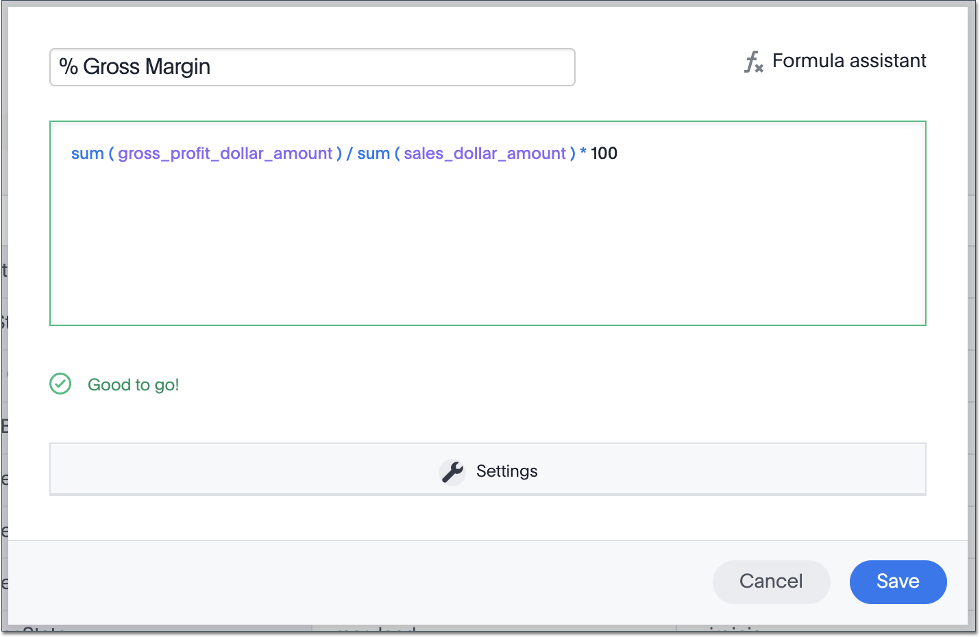
In the top field, enter the formula title: % Gross Margin.
-
In the next field, enter this formula:
sum ( gross_profit_dollar_amount ) / sum ( sales_dollar_amount ) * 100 -
Select Save.
-
-
Save the worksheet with the formula added, by clicking the more options icon
, and selecting Save. -
Select Data, and click the Retail Sales worksheet.
-
In the Columns view, make sure that the % Gross Margin formula has the following settings:
-
For DATA TYPE: DOUBLE
-
For COLUMN TYPE: MEASURE
-
For AGGREGATION: AVERAGE
-
-
Save the worksheet with the updated formula settings, by clicking the more options icon
, and selecting Save.
Best practices for worksheets
The best practices for data modeling also apply to worksheets.
The example here includes:
-
Changed column names
-
Synonyms for columns
-
% Gross Margin formula
image::partner-connect-worksheet-best.png[Worksheet with changed column names, synonyms for columns, and a % gross margin formula]
Adding a currency and geo map to a worksheet
To further enhance the usability of a worksheet, you can add a specific currency type to monetary values, and a geographic map to regions in your data.
Using the Retail Sales worksheet example, here’s how geo maps and currency could be added:
-
Select Data, and click the Retail Sales worksheet.
-
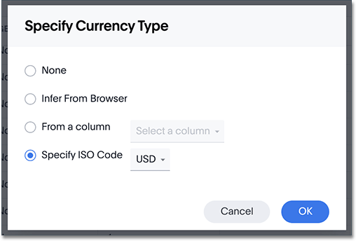
In the Columns view, find the Sales column and select None in the Currency Type column.
-
In the Specify Currency Type window, select Specify ISO Code and, then select USD from the dropdown menu.
-
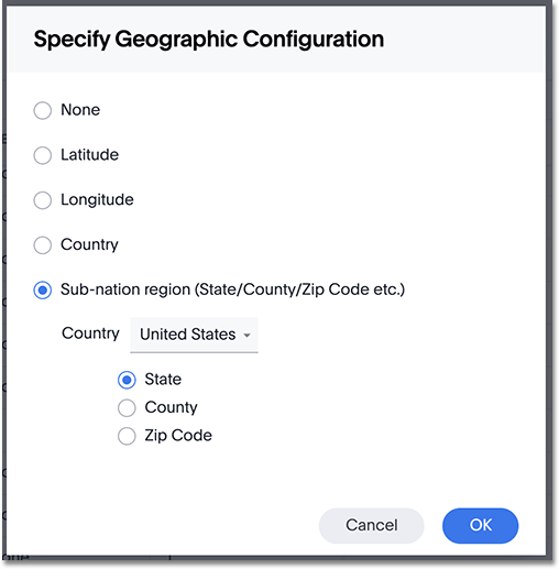
In the Columns view, find the Store_State column, and select None in the Geo Config column.
-
In the Specify Geographic Configuration window, select Specify Sub-nation region, keep the default country of United States, and then select State.
-
Select Save Changes.
Now that both currency and geographic types are set, you can see those changes reflected when you search the Retail Sales worksheet.
-
Select Search.
-
Select Choose sources.
-
Deselect any tables previously selected (if needed), select only the Retail Sales worksheet, and click Close.
-
In the search bar, enter: sales store state and press tab.
The initial search results appear, but without labels for each state.
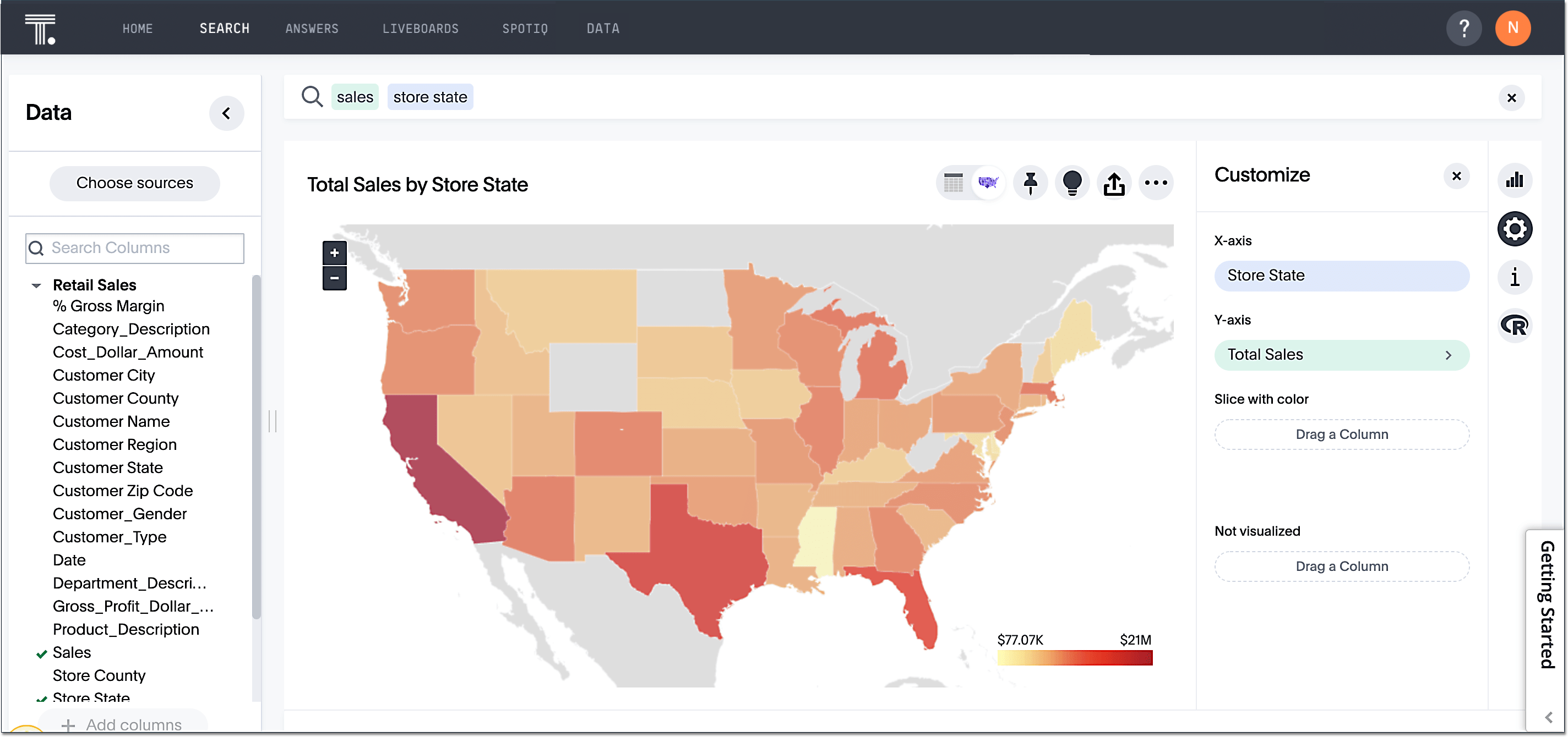
The final step is to add the labels.
-
Select the Edit chart configuration icon
 .
. -
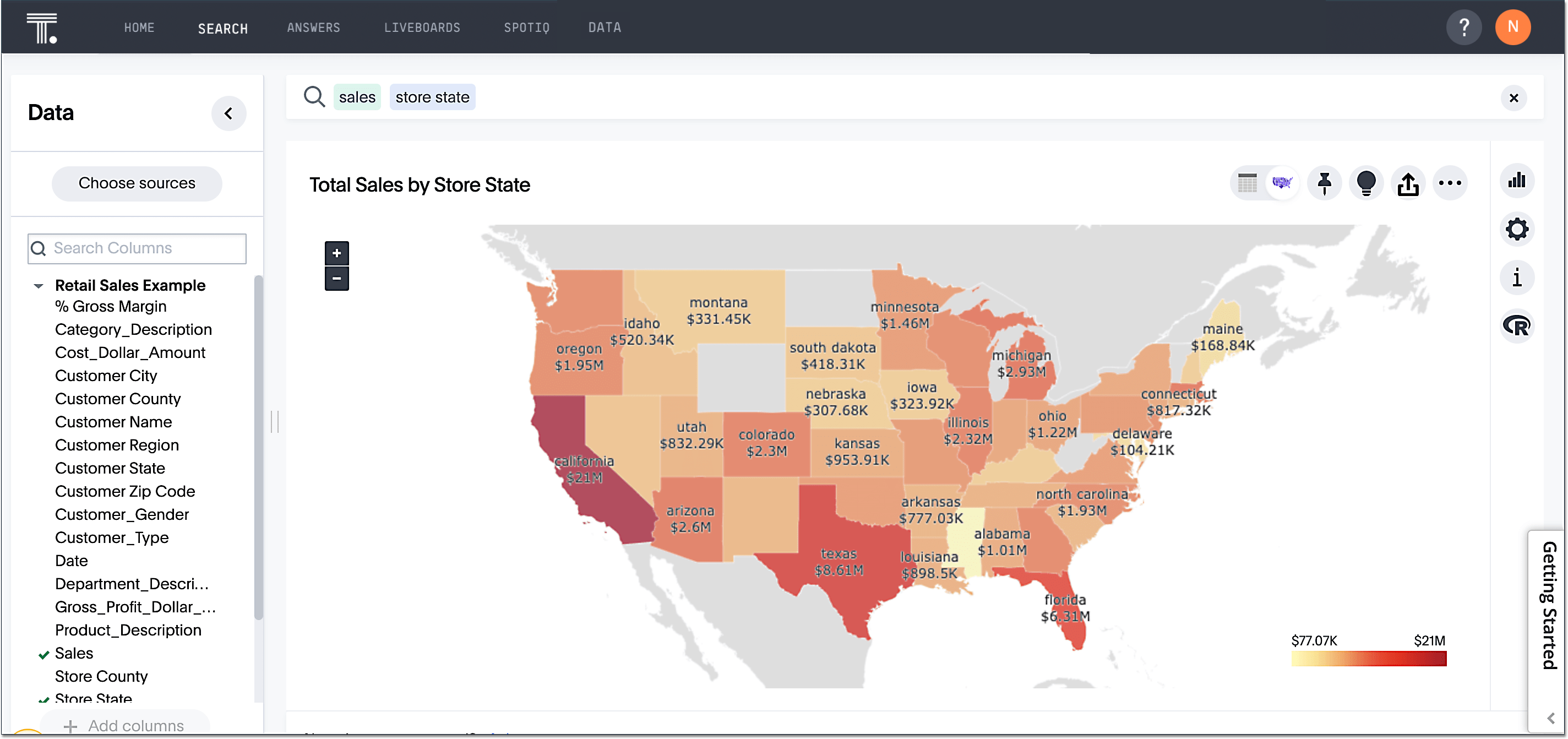
In the Customize panel, select the Total Sales tile.
-
In the Edit column panel, select the Data Labels checkbox.
Now in the search results, you can see labels with the state name and total sales in US dollars.
Related information


